Previous Lesson   All Notes   Next Lesson  

Vector Spaces

In quantum mechanics, the mathematical formalism of vector spaces can simplify problems dramatically. The vector space most people are familiar with is $V^2(\mathbb{R})$. This vector space is a collection of all vectors in the Cartesian $xy$ plane. Both $x$ and $y$ can take any real value, so they are both in $\mathbb{R}$. Since there are 2 separate degrees of freedom $(x,y)$ each vector has 2 components. Hence the vector space is $V^2(\mathbb{R})$. If you’ve ever dealt with complex numbers, you know we often visualize a complex number using a Cartesian plane. A vector space where vectors are 1 dimensional and complex valued, known as $V^1(\mathbb{C})$, has a one-to-one mapping with $V^2(\mathbb{R})$. For the vector $[x,y] \in V^2(\mathbb{R}) $, the corresponding vector in $V^1(\mathbb{C})$ is $[x+iy]$ where $i=\sqrt{-1}$.

Now that you have some examples, here are some formal definitions:

A Field $F$ is a set of scalars which is closed under 2 operations, addition and multiplication. Some examples are the real numbers $\mathbb{R}$ and the complex numbers $\mathbb{C}$. Note that the integers $\mathbb{Z}$ are not a field.

A Vector Space $V(F)$ is a set of vectors closed under 2 operations, vector addition and scalar multiplication. The components of each vector are scalars in the field $F$, and scalar multiplication refers to multiplication only by scalars in $F$.

Linear Independence

The idea of linear independence is crucial in quantum mechanics. Consider the vectors in the picture below:

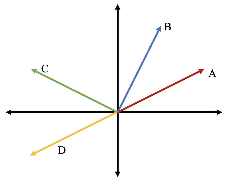
The vectors in this image can be written in $ V^2(\mathbb{R}) $ like

$\vec{A} = \begin{bmatrix} 2 \\ 1 \end{bmatrix}$ $\vec{B} = \begin{bmatrix} 1 \\ 2 \end{bmatrix}$ $\vec{C} = \begin{bmatrix} -2 \\ 1 \end{bmatrix}$ $\vec{D} = \begin{bmatrix} -2 \\ -1 \end{bmatrix}$

where the top number is their length projected on to the horizontal axis and the bottom number is their length projected on to the vertical axis.

If two vectors are linearly independent, then that means you can not make one from the other with multiplication. For example, $\vec{A}$ and $\vec{D}$ are linearly dependent because they are related by scalar multiplication.

\[-1 \cdot \vec{A} = \begin{bmatrix} -2 \\\ -1 \end{bmatrix} = \vec{D}\]

If we tried to do the same process with any other pairing of vectors, there would be no such number. However, the property of linear independence also applies to any set of vectors, not just pairs of vectors. For example, lets take the set of three vectors $\{ \vec{A},\vec{B},\vec{C} \}$. This set is linearly dependent because I can write each vector as a linear combination of the others:

\[\vec{A} = \begin{bmatrix} 2 \\\ 1 \end{bmatrix} = \begin{bmatrix} \frac{4}{5} + \frac{6}{5} \\\ \frac{8}{5} - \frac{3}{5} \end{bmatrix} = \begin{bmatrix} \frac{4}{5} \\\ \frac{8}{5} \end{bmatrix} - \begin{bmatrix} -\frac{6}{5} \\\ \frac{3}{5} \end{bmatrix} = \frac{4}{5} \begin{bmatrix} 1 \\\ 2 \end{bmatrix} -\frac{3}{5} \begin{bmatrix} -2 \\\ 1 \end{bmatrix}\] \[\vec{A} = \frac{4}{5} \vec{B} -\frac{3}{5} \vec{C}\]

A linear combination is the addition of scalar multiples of vectors. Because a vector space is closed under vector addition and scalar multiplication, any linear combination of vectors in a vector space will be in that vector space.

There is an important reason we label the vector space $ V^2(\mathbb{R}) $ with a $2$. If we pick two linearly independent vectors (like $\vec{B}$ and $\vec{C}$), we can make any other vector in $ V^2(\mathbb{R}) $ through a linear combination. In fact, we already did this when we wrote out the horizontal and vertical components of the vectors. If we label a horizontal vector of length $1$ as $\hat{x}$ and a vertical vector of length $1$ as $\hat{y}$, then we can write a vector as

\[\vec{A} = 2 \hat{x} + 1 \hat{y}\]

That was why we wrote $\vec{A} = \begin{bmatrix} 2 \\ 1 \end{bmatrix}$

Hilbert space

Hilbert space, or function space, is best explained by first considering that polynomials of power $n$ define their own vector space. In this space $P^n(\mathbb{R})$, every vector can be written as some

\[f(x) = \sum_{i=0}^n a_i x^i\]

where $x, a_i \in \mathbb{R}$. If we take the vector space in the limit of $n\rightarrow \infty$, then we get a Hilbert space. In Hilbert space, every vector is a function. Depending on restrictions we place on the properties of allowed functions in the space, we can get different Hilbert spaces. However, we can just think of Hilbert space as the space of all real-vaued (or complex valued) functions. In general, we will atleast require the functions be continous in quantum mechanics.

Inner product spaces

An inner product space is a vector space which has a well-defined inner product operation. For example, in any vector space $V^n(\mathbb{R})$ of the type we have been working with, the inner product of two vetors $\vec{A}$ and $\vec{B}$ is given by

\[\vec{A} \cdot \vec{B} = \sum_{j} A_j B_j\]

where $A_j$ are the components of the vector $\vec{A}$ in some reference frame. For a Hilbert or function space, the inner product of two real valued functions $f,g$ is generally denoted and defined by

\[\langle f, g \rangle = \int_{\mathbb{R}} dx f(x) g(x)$= \int_{-\infty}^{\infty} dx f(x) g(x)\]

where the integration is over the entire real number line. Often in quantum mechanics, we will use wavefunctions which take a real value and map it to a complex value. In this case, the inner product is

\[\langle f, g \rangle = \int_{-\infty}^{\infty} dx f^*(x) g(x)\]

where $f^*(x)$ is the complex conjugate of $f(x)$.